(You may obtain a PDF version of this lab note at Electrodynamic Geodesics) Note: See also Part 3 of this Lab Note, Gravitational and Electrodynamic Potentials, the Electro-Gravitational Lagrangian, and a Possible Approach to Quantum Gravitation, which contains further development.
1. Introduction It has been understood at least since Galileo’s refutation of Aristotle which legend situates at the Leaning Tower of Pisa, that heavier masses and lighter masses similarly-disposed in a gravitational field will accelerate at the same rate and reach the ground after identical times have elapsed. Physicists have come to describe this with the principle that the “gravitational mass” and the “inertial mass” of any material body are “equivalent.” As a material body becomes more massive and so more-susceptible to the pull of a gravitational field (back when gravitation was viewed as action at a distance), so too this increase in massiveness causes the material body in equal measure to resist the gravitational pull. By this equivalence, the result is a “wash,” and so with the neglect of any air resistance, all the bodies accelerate and fall at the same rate. (The other consequence of Galileo’s escapade, is that it strengthened the role of experimental testing, in relation to the “pure thought” upon which Aristotle had relied to make the “obvious” but untested and in fact false argument that heavy objects should fall faster. In this way, it spawned the essence of what we today know as the scientific method which remains a dynamic blend of thought and creativity, with experience and cold, hard numbers derived from measurement of masses, lengths, and times.)
Along his path to developing the General Theory of Relativity (GTR), Albert Einstein made a brief stop in 1911 in an imaginary elevator, to conduct a gedanken in which he concluded that the physical experience of an observer falling freely in a gravitational field before terminally hitting the ground is no different from what was commonly thought of as Newton’s inertial motion in which a body in motion remained in motion unless acted upon by a “force.” (GTR later showed that this was not quite true, the “asterisk” to this insight arising from the so-called tidal forces.) And, he concluded that the force one feels standing on the floor of an elevator in free fall to which a constant force is then applied, is no different from the force one feels when standing on the surface of the earth.
The General Theory of Relativity, in the end, captured inertial motion and its close cousin of free-fall motion in a gravitational field, in the most elegant way, as simple geodesic motion in a curved geometry along geodesic paths which coincide precisely with the paths one observes for bodies moving under gravitational influences. This was a triumph of the highest order, as it placed gravitational theory on the completely-solid footing of Riemannian geometry, and became the “gold standard” against which all other physical theories are invariably measured, even to this day. (“Marble and wood” is another oft-employed analogy.)
However, the question of “absolute acceleration,” that is, of an acceleration which is not simply a geodesic phenomenon of unimpeded free fall through a swathe carved out by geometry, but rather one in which an observer actually “feels” a “force” which can be measured by a “weight scale” in physical contact between the observer and that body which applies the force, is in fact not resolved by GTR. To this day, it is hotly-debated whether or not there is such a thing as “absolute acceleration.” Surely, the forces we feel on our bodies in elevators and cars and standing on the ground are real enough, but the question is whether there is some way to understand these forces — which are impediments to what would otherwise be our own geodesic free fall motion in spacetime under the influence of gravity and nothing more — as geodesic forces in their own right, simply of a different, supplemental, and perhaps more-subtle character than the geodesics of gravitation. That is the central question to be examined in this lab note.
If we think of the “gravitational mass” of a material body more generally as its “interaction mass” for the specific circumstance in which the “interaction” is “gravitational,” then the answer to the question whether the real forces we feel when our bodies are “absolutely” accelerated might still be described in terms of geometric geodesics, may still lurk amidst Galileo’s legendary escapade at Pisa, but with a twist. In this situation, the “interaction mass” of a material body is now inequivalent to its “inertial mass,” because that interaction is now “electrical” rather than “gravitational.” Here, Aristotle has his day, because “electrically-heavier” bodies do fall faster than “electrically-lighter” ones.
How do electrical masses now come into play? When we fail to maintain our gravitational geodesic motion by failing to morph through the floor of the elevator, or when we fail to continue our gravitational free fall by not falling unimpeded through the earth’s surface, it is because we are stopped by the collective electrical repulsion between billions of electrons in our bodies and billions more in the elevator floor or the earth’s ground. It is because the electrical interaction has now trumped the gravitational interaction and taken us off of our gravitational geodesics. Or, perhaps, if we can obtain a geometric insight into electrodynamics, it is because we are now leaving the gravitational geodesic, and the atoms in our body are instead embarking upon a different sort of geodesic path which now coincides with the path that has long been observed as the Lorentz force motion of a charged mass in an electromagnetic field.
In light of the quantum revolution of the 20th century, one other consideration is in order. In this discussion, we are talking not about quantum phenomenon, but about bulk phenomenon which lend themselves to completely classical description. In the same way that a bulk material body follows a geodesic path through gravitation, the question we raise is whether bulk electrical bodies, or large numbers of electrons in an electric field, can also be understood, via their Lorentz force motion, to be following geodesic paths made of “marble” no less fine than the marble with which General Relativity directs the paths of material bodies through spacetime geometry in a manner that coincides precisely with what we observe and measure to be a gravitational path. We want to understand why we don’t fall through the elevator or through the earth. Not only do we want to understand this in a way that avoids contradicting the geodesic principles of gravitation, we want to do so in a way that seamlessly extends these principles in a totally-self consistent way, into the electromagnetic arena.
Five-dimensional theories (or higher), have frequently been a foundation upon which to try to merge classical gravitation with classical electrodynamics. Kaluza and Klein began the trend, Einstein looked favorably on the effort, many others have followed, but to this day, there is as yet no theory which has been fully compelling in all aspects, and which at the same time, is motivated to a fifth dimension in a completely natural way, conservatively based on solid principles of observational physics which are already firmly-established.
2. Using Dirac’s “Gamma-5” to Motivate a Fifth, Timelike Dimension
One of the most important connections in all of physics is given by the Dirac relationship:

whereby the Dirac 


Also made of “marble,” is the axial Dirac matrix first motivated by Weyl:

which is defined from matrix-multiplying the other four Dirac matrices, and which has a well-established and rigorously-observed physical meaning in relation to the left- and right-chiral handedness of elementary fermions. We know that when the 


We will now motivate a five-dimensional spacetime, based on (2.1) and (2.2), in the following way: The five-dimensional spacetime we employ will be one which is defined as a geometry in which 


The metric tensor for such a five-dimensional geometry, must therefore be formed from the anticommutator of all five of the 

Given the well-known anticommutation properties of the five 


We next define infinitesimal coordinate intervals in the usual way, including a fifth 


Geometrically, in light of the two timelike dimensions, it will often be very useful to regard time not as a “time line” but as a “time plane.” Thus, following Feynman, we might not only think about worldlines which move forwards and backwards in time, but also which move sideways in time, and at various angles through the time plane. In fact, it is particularly helpful if one draws a vertical coordinate axis for ordinary time 
The next step is to specify a metric interval 


(As an aside, for completeness, having extended 


These 

3. A Possible Geometric Interpretation of Rest Mass
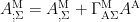
In applying (2.4), we extend all of the customary GTR relationships from four to five dimensions. Thus, 


Now, let’s use algebraic manipulation to rewrite (2.4) in both of the following forms:


Using a velocity four-vector 

If we define a momentum four-vector 


We can capture this very-telling correspondence, by writing:

That is, in some way to be further determined, the rest mass of a material body appears to be proportional to the ratio of 

4. The Geodesic Equation in Five Dimensions
The five-dimensional calculation to follow is analogous to one way of deriving the geodesic equation in four dimensions, though we will in any event carry out the calculation in full a) to help the reader review the basic role of the metric equation as the first integral of the equation of motion b) to convince the reader that the 5-D geodesic equation is in fact correct, and c) to establish a careful discipline about working in five dimensions, making sure that all of our calculations are carried out in a 5-covariant rather than only a 4-covariant manner.
We return to the metric equation (2.4), and now rewrite this, again via trivial algebraic rearrangement, as:

Taking the covariant derivative of each side, employing 

The covariant derivative 


Finally, we contract the 


This looks just like the four-dimensional equation, but for the indexes summing over all five dimensions rather than four, and the 
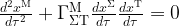
Now, let us work with (4.5) above.
Equation (4.5) is a set of five independent equations. Let’s separate it into the four spacetime equations represented by:

and the single axial-dimension equation:

Equation (4.6) is for 


which on account of

5. Geodesic Motion of a Charged Mass in an Electromagnetic Field
Now, it is time to contrast (4.9) above to the Lorentz Force Law when taken together with the gravitational geodesic equation. This is, for example, set forth in equation (20.41) of Gravitation by Misner, Wheeler and Thorne:

At the outset, let us set aside the term 


Now, we contrast (5.1) directly with (5.2).
The term 


Combining (3.4), 

In fact, if we substitute the proportionalities in (5.3) and (5.4) into (5.1) as if they were equalities, then the geodesic equation (5.2), totally-based in geometry, is the Lorentz force law. Lorentz force motion now appears to be motion along a geodesic, just like gravitational motion. Additionally, this geodesic motion appears to introduce an absolute acceleration, and hence “force,” because of the inequality of electrical and inertial mass, which via (5.3) has its origins in the geometric statement 
In fact, let’s take this geometric understanding of inertial mass and electric charge even a step further. Consider a material body viewed at rest, by setting 

Further, take the weak field approximation where 


Draw 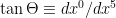


In this way, gravitational and inertial mass, as well as electric mass (charge), obtain a totally geometric interpretation in terms of the angle of a worldline through the time plane. Referring especially to (5.9), movement through ordinary time
6. Symmetric Gravitation and Antisymmetric Electrodynamics: Can they be Compatible?
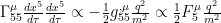
Now, let us turn back to the association 
As it stands, 


So, going into 5-D, and using 

Although unconcerned for now about the extra components in 
Combining

This lets us express the antisymmetric field strength relation
From (6.2), we can rename indexes and use the symmetry of the metric tensor to write:

which further reduces with some index changes and the symmetry of the metric tensor to:
This is an alternative way of saying that
We can further simplify this using the inverse relationship 


The above,
7. Do Maxwell’s Equations Become Components of Einstein’s Gravitational Field Equation?
We have shown the possibility that Lorentz force motion might be described as simple geodesic motion in a five-dimensional spacetime with axial time, and that the inequality of electrical and inertial mass which causes one to “feel” a force and prevents one from falling through the floor of Einstein’s elevator or into the earth’s core, may well emanate from the simple proportionality 
To complete the field theory which we have motivated thus far, one therefore would also need to also examine the Einstein equation in five dimensions:

as well as the Riemann Identity:

to see if among their new axial (index = 5) components, one might find the Maxwell equations 

In five dimensions, one would of course specify the Riemann tensor in the usual way, albeit with an extra “5” index. That is:

Now, let’s consider the 

The second term in the above, with explicit substitution of 
![\Gamma ^{{\rm A} } _{{\rm B} {\rm N} ,5} ={\tfrac{1}{2}} \left[g^{{\rm A} \Sigma } \left(g_{\Sigma {\rm B} ,{\rm N} } +g_{{\rm N} \Sigma ,{\rm B} } -g_{{\rm B} {\rm N} ,\Sigma } \right)\right]_{,5} =0](https://s0.wp.com/latex.php?latex=%5CGamma+%5E%7B%7B%5Crm+A%7D+%7D+_%7B%7B%5Crm+B%7D+%7B%5Crm+N%7D+%2C5%7D+%3D%7B%5Ctfrac%7B1%7D%7B2%7D%7D+%5Cleft%5Bg%5E%7B%7B%5Crm+A%7D+%5CSigma+%7D+%5Cleft%28g_%7B%5CSigma+%7B%5Crm+B%7D+%2C%7B%5Crm+N%7D+%7D+%2Bg_%7B%7B%5Crm+N%7D+%5CSigma+%2C%7B%5Crm+B%7D+%7D+-g_%7B%7B%5Crm+B%7D+%7B%5Crm+N%7D+%2C%5CSigma+%7D+%5Cright%29%5Cright%5D_%7B%2C5%7D+%3D0&bg=ffffff&fg=000000&s=0&c=20201002)
This is equal to zero, as a consequence of

consisting of only three terms.
Now, we make use of 

What is absolutely fascinating, and of enormous eventual import, is that this expression for the mixed field strength tensor 

First, let’s contract (7.7) down to the Ricci tensor, and use the proportionality liberally to eliminate the minus sign, as such:
where 


Note that 


Now, we can return to Einstein’s equation (7.1), for 


This is the first of Maxwell’s equations, for the field of an electric charge. We find, in particular, that 

What about Maxwell’s magnetic equation? Here, we lower all indexes in (7.7) and then use the symmetry 

Then, we turn to some more geometric “marble,” namely the Riemann identity (7.2). Taking the

We may then consider the spacetime subset equations, to write:

Now, Maxwell’s magnetic equation also rests on geometric “marble.”
Maxwell’s electrodynamics in this manner, becomes fully unified with Einstein’s gravitation. The equation for an electric source, 
The magnetic equation 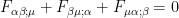

Finally, the geodesic equation 
(We note, as an aside, that 


Irrespective of the ultimate disposition of

Hi Jay,
by tag surfing i stumbled over your blog and i will most likely return. Very interesting ideas and you are certainly able to present them arrestingly.
I had not the time to read the whole entry, but you use the 5th gamma matrix to get a 5-dimensional representation of the clifford algebra. We use the same approach in the Randall-Sundrum Mmodel. The problem we encounter is that because of this in odd dimensional spacetime there is no projection operator. So we are not able to define chiral fermions. We deal with this by orbifolding the extra dimension. I don’t want to explain this further. Just to draw your attention on the problem… you probably already thought about.
keep up the good work.
-martin
Comment by martinbauer — February 6, 2008 @ 11:19 am |
Hi Martin:
I presume the chiral projection operators you refer to are 1 +/- gamma^5? But I am not sure why these would be thought to disappear in an odd-dimensional spacetime.
Would you please send me or point out, something that pinpoints the root of the problem you have in mind, and I’ll see if perhaps some solution seems apparent.
Thanks,
Jay.
email to: jyablon@nycap.rr.com
Comment by Jay R. Yablon — February 6, 2008 @ 6:57 pm |
Hi Jay,
You will not be able to build these projection operators in odd spacetimes. Generally is defined as the product of all “lower” gammas. This gives a projection operator for even dimensional spacetime and 1 for odd dimensions (it’s
  in 5 dimensions).
So or vice versa. You could use the “old”
  to build it, but then again you need
 ![\left[\gamma _{5} ,\gamma _{\mu } \right]=0](https://s0.wp.com/latex.php?latex=%5Cleft%5B%5Cgamma+_%7B5%7D+%2C%5Cgamma+_%7B%5Cmu+%7D+%5Cright%5D%3D0&bg=ffffff&fg=000000&s=0&c=20201002) to get kinetic terms in the lagrangian which couple left handed fermions to left handed , but you already have
to get kinetic terms in the lagrangian which couple left handed fermions to left handed , but you already have  .
.
In your case, its even worse. Cause …
…
You can look it up at sundrums lecture : http://arxiv.org/abs/hep-th/0508134
theres is some supersymmetry book also, but i cant remember which one right now. will tell you later.
martin
Comment by martinbauer — February 7, 2008 @ 6:07 am |
To do the dirty deed in an odd spacetime you can add an extra degree of freedom to the Clifford algebra that is not a part of the algebra. Replace the four gamma matrices with the symbols x, y, z, t to allow me to avoid tex. Add a fifth gamma matrix s.
Sure enough, the product xyzst is an object that squares to +1 and commutes with everything in the algebra. It’s natural to assume that it is therefore equal to 1 but you don’t have to do that. This is entirely up to the user. Personally, I think you should leave it as a non unit and that makes (1 +- xyzst)/2 perfectly good as a projection operator.
An alternative construction, and one that I worked with for quite some time, is to begin with an even Clifford algebra, like the Dirac algebra with x, y, z, and t, and add a single extra degree of freedom to it. The extra degree of freedom is assumed to commute with everything else in the algebra and square to 1. That will give you an algebra that is isomorphic to that generated by {x,y,z,s,t} and it explicitly defines the (1+xyzst)/2 projection operator as non trivial.
Eventually an expert on the geometric algebra versions of Clifford algebra pointed out to me that what I was doing was isomorphic to the usual C(4,1) so I quit doing that and just used C(4,1) instead. They make perfectly good projection operators.
It is also easy to give a physical justification for adding an extra degree of freedom that commutes with everything else in the algebra. Suppose you wish to define a theory that has non commutative degrees of freedom for the spatial components but is Newtonian in that time is not included in with the spatial degrees of freedom. The natural number of dimensions to take is 3. For the spatial degrees of freedom you get the Pauli algebra.
The Dirac algebra arose from looking for a square root for the Klein-Gordon equation. The massless Klein-Gordon (which is appropriate for theories that split the particles into massless chiral halves) arises naturally in perfectly Newtonian circumstances without spacetime. For example, earth quake waves are governed by it. In this case, the time coordinate is not a part of the geometry, so when you take a square root of it, there’s no (relativistic) motivation to make the time coordinate act like the others. However, the massless Klein-Gordon equation (and any other wave equation) needs two degrees of freedom in time. So if you do not treat time like space you will instead have to split it into two equations that are distinct and coupled. They look something like this:
[tex]D \psi = \phi, D\phi = \psi[/tex]
where D is your Dirac operator without a gamma_0. So this means that instead of using just psi or phi, what you end up with is a vector that contains \psi and \phi as separate components. To melt them into the same object, just define a commuting vector “T” which satisfies TT = 1, and write [tex]\Psi = \psi + T\phi[/tex]. Then you can take the above two coupled linear equations and combine them into a single linear equation:
[tex]D \Psi = 0[/tex]
In doing this, you can use the projection operators (1 +- T)/2 to split the \Psi back into its components. It’s perfectly physical, correct mathematically, and there is nothing wrong with it, rock on.
Comment by carlbrannen — February 11, 2008 @ 12:58 pm |
[…] Note: This Lab Note picks up where Lab Note 2, Part 2, left off, following section 7 thereof. Equation numbers here, reference this earlier Lab […]
Pingback by Lab Note 2, Part 3: Gravitational and Electrodynamic Potentials, the Electro-Gravitational Lagrangian, and a Possible Approach to Quantum Gravitation « Lab Notes for a Scientific Revolution (Physics) — February 14, 2008 @ 1:39 am |
Hi Martin:
As regards your comment #3, I was curious if you felt that Carl provided a satisfactory answer in #4? (I will try to decipher and fix your “does not parse” equations.)
Just saw your new post over at http://martinbauer.wordpress.com/. Your analogy to pirates looking for treasure and not having a great map is a good one.
Carl, by the way, has is own blog over at http://carlbrannen.wordpress.com/.
Best regards,
Jay,
Comment by Jay R. Yablon — February 14, 2008 @ 11:00 am |
Hi Martin:
I fixed up your non-printing latex equations in comment #3. I understand all you said, but don’t see a problem. Maybe I am missing something, but here is how I see it:
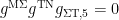
I am using a 5-D metric tensor . (Though I work with curved
  , the Minkowski metric tensor will suffice for this discussion.)
You say “Generally is defined as the product of all “lower” gammas.” Do I take this to mean that in 5-D, I have to define yet another
  and use this for projections?
You say “This gives a projection operator for even dimensional spacetime and 1 for odd dimensions (it’s in 5 dimensions).” Exactly how do you calculate that the projection operator is
  in 5 dimensions?
I looked at Sundrum’s lecture at http://arxiv.org/abs/hep-th/0508134 . Thanks for the link. In his (3.1), he defines Presumably, this is to force a spacelike signature upon the fifth dimension, i.e., + – – – -, which seems to be the penchant in 5-D theories. I just go with the flow and use the “old”
  , which is what accounts for my + – – – + signature, i.e., for a timelike fifth dimension. As my paper shows, there are advantages that arise from a second timelike dimension, including the fact that mass and charge can be characterized by virtue of their “angle” of travel through time and we can specify the Lorentz force law as geodesic motion, etc. Does that difference perhaps account for the problem you are envisioning? It looks like it does, because, e.g.,
  and
and  are very different projection terms than
  and
and  , and the latter get real funny when you take complex conjugates.
You say “You could use the “old” to build it,” and in fact, I do simply use the old
  as the projection in the usual way. Why not? That is:
  as always. I define
  and
and  , as always. Thus, when we project from a Fermion wavefunction
  , we have
  and
and  . Is there a reason why I am compelled not to make these choices?
The adjoint is , and, of course,
  . So,
. So,  and
and  . Then, the Fermion couplings work as follows:
When there is no sandwiched,
  and
and  which uses
  and
and  . Further,
  and
and  , which uses
  .
.
When there is a sandwiched, then
  and
and  . Further,
  and
and  .
.
All of this seems as it should be, to me. Can you please point out where I might be missing something?
Thanks,
Jay.
Comment by Jay R. Yablon — February 14, 2008 @ 12:23 pm |
Hi Carl and Jay,
First, there s a mistake in my first comment. You can delete the 5th sentence.
The question is: are there chiral representations of the Clifford algebra in odd spacetime dimensions (p+q=n odd, no matter how many spaces, times). And the answer is simple : There are none.
you can look it up in a lot of books (i.e. Cornwell has an exhaustive discussion in the appendix ).
You need another, fifth , 4×4 matrix, anticommuting with each you already have. It is easy to check that the only possibility you have is to use some multiple of
  , a some c-number. So
  is part of your dirac algebra already.
Now you try to define projections. To define projection operators you need a 4×4 matrix anticommuting with all (also
(also  now). There is no such matrix left (= no additional degree of freedom thats not part of the algebra) . That is, because the Clifford algebra provides a basis for the space of 4×4 real matrices. If there’d be another it would be a linear-combination, plus the demand to anticommute with all the others –> it needs to be a product of all
  , therefore
  .
.
you can’t use the old . It commutes with
  (jay, all your calculations fail if you put
  ).
). as you said above will yield
  (another way: it will commute with every element of the algebra and is therefore 1 by Schurs lemma).
Try to define a
Carl, the expert on geometric algebra must be joking with you, or he is far from beeing an expert. C(4,1) as every other clifford algebra (group) over an odd spacetime does not allow for a projective operator.
To have chiral fermions you need even spacetime dimension or orbifolding the extradimension.
Best,
martin
Comment by martinbauer — February 15, 2008 @ 1:16 pm |
Hi Martin, Thanks for your comment #8. The Cornwell link is in error — it points to one of my own posts. Can you please provide a corrected link. Thanks. Jay.
PS: Update: Martin sent me a corrected link to Cornwell, now fixed in #8. Jay.
Comment by Jay R. Yablon — February 15, 2008 @ 4:54 pm |